"Event stereo matching is an emerging technique to estimate depth from neuromorphic cameras; however, events are unlikely to trigger in the absence of motion or the presence of large, untextured regions, making the correspondence problem extremely challenging. Purposely, we propose integrating a stereo event camera with a fixed-frequency active sensor -- e.g., a LiDAR -- collecting sparse depth measurements, overcoming the aforementioned limitations. Such depth hints are used by hallucinating -- i.e., inserting fictitious events -- the stacks or raw input streams, compensating for the lack of information in the absence of brightness changes. Our techniques are general, can be adapted to any structured representation to stack events and outperform state-of-the-art fusion methods applied to event-based stereo."

1 - Problems

1. Given a pair of stereo event streams, deep event stereo networks try to estimate a dense disparity map from the stacked event streams. However, the latter are uninformative when facing large uniform areas or in the absence of motion: consequentially, event stereo networks struggle to match events across left and right cameras.

2. Several techniques (e.g., LidarStereoNet, Guided Stereo Matching, VPP) uses a synchronous depth sensor, such as a LiDAR, to alleviate this problem in the RGB literature, however, a simple porting of those techniques is not trivial since the fixed-frequency rate of LiDARs is in contrast with the asynchronous acquistion rate of event cameras. This would case to either i) use depth points only when available, harming the accuracy of most fusion strategies known from the classical stereo literature, or ii) limiting processing to the LiDAR pace, nullifying one of the greatest strength of event cameras -- i.e., microseconds resolution. Nonetheless, this track on event stereo/active sensors fusion has remained unexplored so far.

   Event cameras vs LiDARs -- strengths and weaknesses. Event cameras provide rich cues at object boundaries where LiDARs cannot (cyan), yet LiDARs can measure depth where the lack of texture makes event cameras uninformative (green).

2 - Proposal

1. Inspired by our previous proposal VPP, we design a hallucination mechanism to generate fictitious events over time to densify the stream collected by the event cameras. Purposely, we propose two different event-depth fusion strategies:

   1. creating distinctive patterns directly at the stack level, i.e. a Virtual Stack Hallucination (VSH), just before the deep network processing;
   2. generating raw events directly in the stream, starting from the time instant td for which we aim to estimate a disparity map and performing Back-in-Time Hallucination (BTH).

   Overview of a generic event-based stereo network and our hallucination strategies. State-of-the-art event-stereo frameworks (a) pre-process raw events to obtain event stacks fed to a deep network. In case the stacks are accessible, we define the model as a gray box, otherwise as a black box. In the former case (b), we can hallucinate patterns directly on it (VSH). When dealing with a black box (c), we can hallucinate raw events that will be processed to obtain the stacks (BTH).

2. Furthermore, despite depth sensors having a fixed acquisition rate thatis in contrast with the asynchronous capture rate of event cameras, VSH and BTH can leverage depth measurements not synchronized with $t_d$ (thus collectedat $t_z < t_d$) with marginal drops in accuracy compared to the case of perfectly synchronized depth and event sensors ($t_z = t_d$). This strategy allows for exploiting both VSH and BTH while preserving the microsecond resolution peculiar of event cameras.

3 - Hallucinations

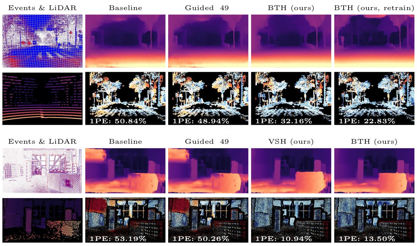
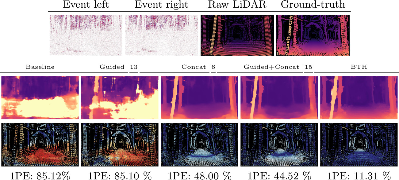
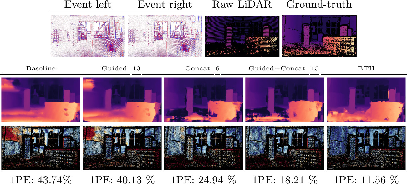
According to the sensor fusion literature for conventional cameras, the main strategies for combining stereo images with sparse depth measurements from active sensors consist of i) concatenating the two modalities and processing them as joint inputs with a stereo network, ii) modulating the internal cost volume computed by the backbone itself or, more recently, iii) projecting distinctive patterns on images according to depth hints. We follow the latter path, since it is more effective and flexible than the alternatives -- which can indeed be applied to white box frameworks only. For this purpose, we design two alternative strategies suited even for gray and black box frameworks.

• Virtual Stack Hallucination -- VSH: Given left and right stacks $\mathcal{S}_L,\mathcal{S}_R$ of size W$\times$H$\times$C and a set $Z$ of depth measurements $z(x,y)$ by a sensor, we perform a Virtual Stack Hallucination (VSH), by augmenting each channel $c\in\text{C}$, to increase the distinctiveness of local patterns and thus ease matching. This is carried out by injecting the same virtual stack $\mathcal{A}(x,y,x',c)$ into $\mathcal{S}_L,\mathcal{S}_R$ respectively at coordinates $(x,y)$ and $(x',y)$. $$\mathcal{S}_L(x,y,c) \leftarrow \mathcal{A}(x,y,x',c)$$ $$\mathcal{S}_R(x',y,c) \leftarrow \mathcal{A}(x,y,x',c)$$ with $x'$ obtained as $x-d(x,y)$, with disparity $d(x,y)$ triangulated back from depth $z(x,y)$ as $\frac{bf}{z(x,y)}$, according to the baseline and focal lengths $b,f$ of the stereo system. We deploy a generalized version of the random pattern operator $\mathcal{A}$ proposed in VPP, agnostic to the stacked representation: $$\mathcal{A}(x,y,x',c) \sim \mathcal{U}(\mathcal{S}^-, \mathcal{S}^+)$$ with $\mathcal{S}^-$ and $\mathcal{S}^+$ the minimum and maximum values appearing across stacks $\mathcal{S}_L,\mathcal{S}_R$ and $\mathcal{U}$ a uniform random distribution. Following VPP, the pattern can either cover a single pixel or a local window. This strategy alone is sufficient already to ensure distinctiveness and to dramatically ease matching across stacks, even more than with color images, since acting on semi-dense structures -- i.e.,, stacks are uninformative in the absence of events. It also ensures a straightforward application of the same principles used on RGB images, e.g.,, to combine the original content (color) with the virtual projection (pattern) employing alpha blending. Nevertheless, we argue that acting at this level i) requires direct access to the stacks, i.e., a gray-box deep event-stereo network, and ii) might be sub-optimal as stacks encode only part of the information from streams.

• Back-in-Time Hallucination -- BTH: A higher distinctiveness to ease correspondence can be induced by hallucinating patterns directly in the continuous events domain. Specifically, we act in the so-called event history: given a timestamp $t_d$ at which we want to estimate disparity, raw events are sampled from the left and right streams starting from $t_d$ and going backward, according to either SBN or SBT stacking approaches, to obtain a pair of event histories $\mathcal{E}_L = \left\{ e^L_k \right\}^{N}_{k=1}$ and $\mathcal{E}_R = \left\{ e^R_k \right\}^{M}_{k=1}$, where $e^L_k,e^R_k$ are the $k$-th left and right events. Events in the history are sorted according to their timestamp -- i.e.,, inequality $t_k \leq t_{k+1}$ holds for every two adjacent $e_{k},e_{k+1}$. At this point, we intervene to hallucinate novel events: given a depth measurement $z(\hat{x},\hat{y})$, triangulated back into disparity $d(\hat{x},\hat{y})$, we inject a pair of fictitious events $\hat{e}^L=(\hat{x},\hat{y},\hat{p},\hat{t})$ and $\hat{e}^R=(\hat{x}',\hat{y},\hat{p},\hat{t})$ respectively inside $\mathcal{E}_L$ and $\mathcal{E}_R$, producing $\hat{\mathcal{E}}_L=\left\{e^L_1,\dots,\hat{e}^L,\dots,e^L_N\right\}$ and $\hat{\mathcal{E}}_R=\left\{e^R_1,\dots,\hat{e}^R,\dots,e^R_M\right\}$. By construction, $\hat{e}^L$ and $\hat{e}^R$ adhere to i) the time ordering constraint, ii) the geometry constraint $\hat{x}'=\hat{x}-d(\hat{x},\hat{y})$ and iii) a similarity constraint -- i.e.,, $\hat{p},\hat{t}$ are the same for $\hat{e}^L$ and $\hat{e}^R$. Fictitious polarity $\hat{p}$ and fictitious timestamp $\hat{t}$ are two degrees of freedom useful to ensure distinctiveness along the epipolar line and ease matching, according to which we can implement different strategies, and detailed in the remainder.

  Overview of Back-in-Time Hallucination (BTH). To estimate disparity at $t_d$, if LiDAR data is available -- e.g., at timestamp $t_z=t_d$ (green) or $t_z=t_d-15$ (yellow) -- we can naively inject events of random polarities at the same timestamp $t_z$ (a). More advanced injection strategies can be used -- e.g., by hallucinating multiple events, starting from $t_d$, back-in-time at regular intervals (b).

  Single-timestamp injection: The simplest way to increase distinctiveness is to insert synchronized events at a fixed timestamp. Accordingly, for each depth measurement $d(\hat{x},\hat{y})$, a total of $K_{\hat{x},\hat{y}}$ pairs of fictitious events are inserted in $\mathcal{E}_L,\mathcal{E}_R$, having polarity $\hat{p}_k$ randomly chosen from the discrete set $\left\{-1,1\right\}$. Timestamp $\hat{t}$ is fixed and can be, for instance, $t_z$ at which the sensor infers depth, that can coincide with timestamp $t_d$ at which we want to estimate disparity -- e.g.,, $t_z=t_d=0$ in the case (a). Inspired by , events might be optionally hallucinated in patches rather than single pixels. However, as depth sensors usually work at a fixed acquisition frequency -- e.g.,, 10Hz for LiDARs -- sparse points might be unavailable at any specific timestamp. Nonetheless, since $\mathcal{E}_L,\mathcal{E}_R$ encode a time interval, we can hallucinate events even if derived from depth scans performed in the past -- e.g.,, at $t_z < t_d$, -- by placing them in the proper position inside $\mathcal{E}_L,\mathcal{E}_R$.

  Repeated injection: The previous strategy does not exploit one of the main advantages of events over color images, i.e., the temporal dimension, at its best. Purposely, we design a more advanced hallucination strategy based on repeated naive injections performed along the time interval sampled by $\mathcal{E}_L, \mathcal{E}_R$. As long as we are interested in recovering depth at $t_d$ only, we can hallucinate as many events as we want in the time interval before $t$ -- i.e.,, for $t_z=t_d=0$, over the entire interval as shown in (b) -- consistent with the depth measurements at $t_d$ itself, which will increase the distinctiveness in the event histories and will ease the match by hinting the correct disparity. We can design a strategy for injecting multiple events along the stream. Accordingly, we define the conservative time range $\left[t^-,t^+\right]$ of the events histories $\mathcal{E}_L, \mathcal{E}_R$, with $t^-=\min\left\{t^L_0,t^R_0\right\}$ and $t^+=\max\left\{t^L_N,t^R_M\right\}$ and divide it into $B$ equal temporal bins. Then, inspired by MDES, we run $B$ single-timestamp injections at $\hat{t}_b=\frac{2^b-1}{2^b}(t^+-t^-)+t^-$, with $b \in \left\{1,\dots,B\right\}$. %$\hat{t}_b=\frac{2^b-1}{2^b}\Delta t+t^-$. Additionally, each depth measurement is used only once -- i.e.,, the number of fictitious events $K_{b,\hat{x},\hat{y}}$ in the $b$-th injection is set as $K_{b,\hat{x},\hat{y}} \leftarrow K_{\hat{x},\hat{y}}\delta(b,D_{\hat{x},\hat{y}})$ where $\delta(\cdot,\cdot)$ is the Kronecker delta and $D_{\hat{x},\hat{y}}\leftarrow\text{round}(X^\mathcal{U}(B-1)+1)$ is a random slot assignment. We will show in our experiment how this simple strategy can improve the results of BTH, in particular increasing its robustness against misaligned LiDAR data -- i.e., measurements retrieved at a timestamp $t_z < t_d$.

Performance versus Competitors

We test the effectiveness of BTH and alternative approaches on DSEC and M3ED, using the backbones trained on DSEC without any fine-tuning on M3ED itself. On DSEC (top), BTH dramatically improves results over the baseline and Guided, yet cannot fully recover some details in the scene except when retraining the stereo backbone. On M3ED (bottom), both VSH and BTH with pre-trained models reduce the error by 5x.

Concat and Guided+Concat can reduce the error by about 40%, yet far behind the improvement yielded by BTH (more than 70% error rate reduction). Our proposal confirms again the best solution for exploiting raw LiDAR measurements and improve the accuracy of event-based stereo networks.

Robustness against time-misaligned LiDAR

We conclude by assessing the robustness of the considered strategies against the use of LiDAR not synchronized with the timestamp at which we wish to estimate disparity -- occurring if we wish to maintain the microsecond resolution of the event cameras. Not surprisingly, the error rates arise at the increase of the temporal distance: while this is less evident with Guided because of its limited impact, this becomes clear with VSH and BTH. Nonetheless, both can always retain a significant gain over the baseline model -- i.e., the stereo backbone processing events only -- even with the farthest possible misalignment with a 10Hz LiDAR (100ms).